Initialisation Benchmark

For our initialisation benchmarks we estimate the time to execute get_unitary_evolver() using pyperf with three values and 20 processes: 60 sample points per data point in the plots below. We fix the number of control Hamiltonians to 10 and vary the vector space dimension in the range \(\left[1, 64\right]\). We benchmark both the static and dynamic evolvers in the range \(\left[1, 16\right]\) and then only benchmark dynamic evolvers there after. For all data points we consider both a dense and a sparse evolver.

Dense Hamiltonian

For the dense test we randomly generate a drift and 10 control Hamiltonians of dimension dim using:

import numpy as np
H = np.random.rand(dim, dim)+1j*np.random.rand(dim, dim)
H = H + H.T.conj()

The results are:

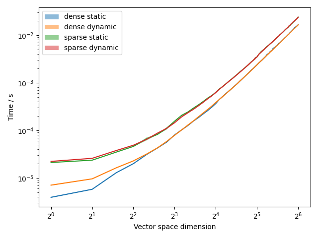
The shaded region indicates plus or minus one standard deviation from the mean.

We can see that the dense evolver outperforms the sparse evolver for dense Hamiltonians. Additionally, we see that the static dense evolver only outperforms the dynamic dense evolver at low vector space dimensions. There is little difference in performance between the sparse static and dynamic evolvers.

Sparse Hamiltonian

For the sparse test we set the drift and all the control Hamiltonians to the identity.

The results are:

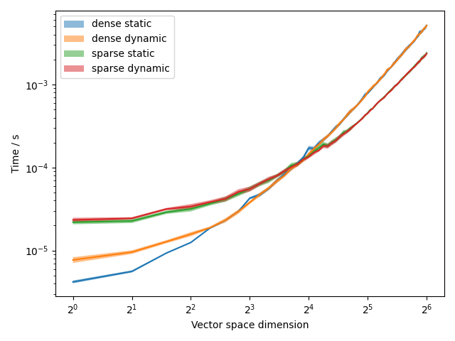
The shaded region indicates plus or minus one standard deviation from the mean.

For sparse Hamiltonians and sufficiently large vector space dimensions the sparse evolvers outperform the dense evolvers. Interestingly all evolvers exhibit a greater variance in runtimes for sparse Hamiltonians. Once again we observe that the dense static evolver outperforms the dense dynamic evolver for small systems but there is little difference for the sparse evolvers.