Propagation Benchmark

For our propagation benchmarks we estimate the time to execute propagate() using pyperf. We fix the number of control Hamiltonians to 10 and vary the vector space dimension (dim) in the range \(\left[1, 64\right]\). We benchmark both the static and dynamic evolvers in the range \(\left[1, 16\right]\) and then only benchmark dynamic evolvers there after. For all data points we consider both a dense and a sparse evolver. propagate() is executed with random control amplitudes and initial state generated by

import numpy
N_CTRL = 10
TIME_STEPS = 100
ctrl_amp = np.random.rand(TIME_STEPS, N_CTRL).astype(np.complex128)
state = np.random.rand(dim).astype(np.complex128)
state /= np.linalg.norm(state)

We use 100 time steps each of duration 0.1.

Dense Hamiltonian

For the dense test we randomly generate a drift and 10 control Hamiltonians of dimension dim using:

import numpy as np
H = np.random.rand(dim, dim)+1j*np.random.rand(dim, dim)
H = H + H.T.conj()

To perform these benchmarks we use three values and five processes: 15 sample points per data point. The results are:

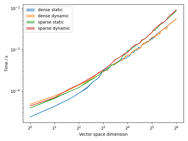
The shaded region indicates plus or minus one standard deviation from the mean.

We observe that for small dimensions the dense static evolver performs best with the other three having little difference between them. At larger dimensions the dense evolvers outperform the sparse evolvers.

Sparse Hamiltonian

For the sparse test we set the drift and all the control Hamiltonians to the identity.

To perform these benchmarks we use three values and 20 processes: 60 sample points per data point. The results are:

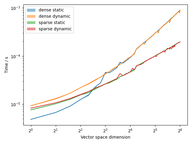
The shaded region indicates plus or minus one standard deviation from the mean.

Similarly to the previous benchmark the dense static evolver performs best at low dimensions. However, the sparse evolvers perform better than the dense dynamic evolver for low dimensions. At large dimensions the sparse evolvers outperform the dense evolvers. The static and dynamic sparse evolvers show little difference in performance.